Georeferencing images like a caveman
I’ve been intrigued by local history and urban development for as long as I can remember. A natural exercise for those who share this interest is georeferencing - overlaying a raster image (such as an old map) on a modern digital map.
I found it frustrating that all the guides for doing this referred to which buttons to press on proprietary software such as ArcGIS or Google Earth. After all, isn’t it basically just about mapping from one two-dimensional coordinate system to another one, using some data points? I set out to do this from scratch.
First, I downloaded a 1910 historical map from Rahvusarhiiv and it is actually the first map of Tallinn printed in the Estonian language.
Using tkinter and opencv, I triggered a simple dialogue box on clicking the raster map, that asks for the latitude and longitude
of the point. I looked up the coordinates from Google Maps, and appended each added point to a .csv file. This generates the
reference points necessary to learn the mapping between the pixels of the raster image and their real life locations.
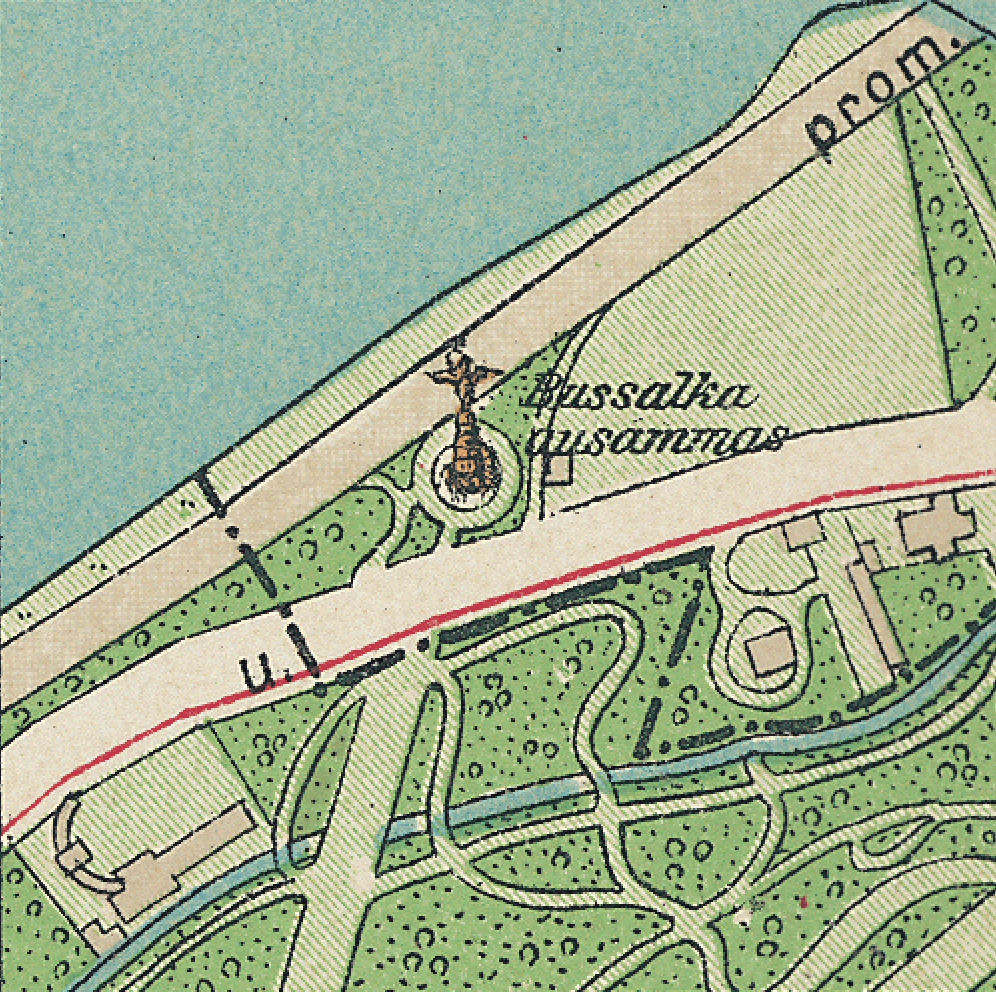
Finding reference points is a fun exercise on its own - essentially you are trying to find bits and pieces of the city that have remained unchanged for 100+ years. It wasn’t too hard for the high definition 1910 map, but proved to be quite tough for a hand drawn map from 1764! For example, the Russalka Memorial in Tallinn was erected in 1902, so it exists on both the 1910 map and today. In a similar manner, old monuments, lighthouses, railway intersections and natural boundaries are your best bet for good reference points.
After collecting the reference points, the next step is to map them. Here comes the caveman part: I simply used two univariate linear regressions on latitude and longitude separately, trying to predict the in-sample coordinates of the references. This worked surprisingly well! The first sign of this is the high R2 coefficient (above 95%) - meaning the simple line drawn through the points captures their variance well.
To actually overlay the raster image correctly on the map, I simply predicted the bounding box of the map, using its four corners as the model input. This implies you’d want to gather enough reference points around the edge of the map (especially with more complex non-linear regressors) for it to fit nicely. I was surprised how well the end result turned up - even though I hadn’t spent any time thinking about map projections, rotation etc. It provided for a smooth viewing experience where toggling between the layers leaves the location more or less intact.
It should be noted that this simple methodology did not work on older maps, probably as combination of it being overly simplistic and the poor quality of maps (at least for Estonia) before the turn of the 20th century.