Effective spatial embeddings for tabular data
I believe the edge of gradient boosted tree models (GBT) over neural networks as the go-to tool for tabular data has eroded over the past few years. This is largely driven by more clever generic embedding methods that can be applied to arbitrary feature inputs, rather than more complex architectures such as transformers. I validate two simple one hot encoding based embeddings that reach parity with GBT on a non trivial spatial problem.
GBT vs DL
Tabular data is one of the few last machine learning strongholds where deep learning does not reign supreme. This is not due to lack of trying, as there have been multiple proposed architectures, maybe the most known being TabNet. What the field lacks though, are generic go-to implementations that would achieve competitive performance on a range of benchmarks, in a similar way as gradient boosted tree ensembles (XGBoost, LightGBM, Catboost - GBT for short) can do. Indeed, Shwartz-Ziv & Armon [4] show that the proposed tabular deep learning methods often outperform others only on the dataset proposed in their papers, generally losing to GBT methods.
Why should we care?
While the GBT vs DL debate can become emotionally loaded at times, there are some objective benefits to the latter approach:
- Seamless online learning. As we generally train deep learning models using minibatches, it is straightforward to extend this to learning continuously on new data, without requiring a full retraining. GBTs cannot fully replicate this, as they are building an increasingly complex additive function. In order to update it, you’d have to either prune the function somehow (e.g. keep only first N trees and add new ones) or keep the tree structure and only update leaf values. Neither can guarantee optimality, while as a neural network is simply a collection of differentiable stacked weight layers, you can fine-tune the whole model.
- Transferability. Closely related to the last point, it means we can reuse a learned model structure and use it for other tasks, or predict multiple things jointly.
- Multimodal inputs. You had a tabular problem? But what if you can use some image data or free form text to improve the accuracy? DL allows to train these kinds of models jointly end to end. That’s much more elegant than combining multiple models (with different APIs) for the same task.
Problem
I’ll use the NYC taxi trip duration dataset from Kaggle and try to predict trip_duration purely as a function of the pickup and dropoff coordinates. This exemplifies a relatively difficult type of tabular problem, as coordinates are numeric features, but we (a) expect to have a non-monotonic relationship between them and the target, with (b) potentially very fine-grained decision boundaries (imagine a city block which has exceptionally restrictive routing), and (c) the target is defined by the interaction of both inputs - trip duration is mostly a function of the distance between pickup and dropoff, so we’re expecting our models to learn this. Additionally, it’s a relevant real life problem for dispatching and logistics planning.
The dataset:
df.info()

<class 'pandas.core.frame.DataFrame'>
RangeIndex: 1458644 entries, 0 to 1458643
Data columns (total 11 columns):
 #   Column              Non-Null Count    Dtype
---  ------              --------------    -----
 0   id                  1458644 non-null  object
 1   vendor_id           1458644 non-null  int64
 2   pickup_datetime     1458644 non-null  object
 3   dropoff_datetime    1458644 non-null  object
 4   passenger_count     1458644 non-null  int64
 5   pickup_longitude    1458644 non-null  float64
 6   pickup_latitude     1458644 non-null  float64
 7   dropoff_longitude   1458644 non-null  float64
 8   dropoff_latitude    1458644 non-null  float64
 9   store_and_fwd_flag  1458644 non-null  object
 10  trip_duration       1458644 non-null  int64
dtypes: float64(4), int64(3), object(4)
memory usage: 122.4+ MB
Basic setup
The regression models are trained for MAE, using early stopping. For the neural networks, learning rate reduction on reaching a plateau is applied. The holdout test set is split by timestamp, to avoid unexpected leakage.
Models
LightGBM
The interaction-based coordinate problem does not really pose a problem for a GBT model. It can perform splits on the lat/lng space as it would on any other numeric feature. By alternating between splits on both pickup and dropoff, it encodes the interaction seamlessly. The only drawback of GBTs for this problem is that the binary splits can only be horizontal or vertical, and that you’d need 4 depth-wise splits to model a square (which in our problem can be relevant neighbourhood). It should be noted that there has been work to extend GBT to spatial splits, e.g. [3], but that’s not available to the lay practitioner.
The obvious argument speaking for models like XGBoost or LightGBM is how easy it is to get started with them and achieve competitive accuracy. Just look at the code below, you do not need to be a data scientist to run this!
lgb_train = lgb.Dataset(X_train, y_train)
lgb_eval = lgb.Dataset(X_valid, y_valid, reference=lgb_train)

model = lgb.train(params,
            lgb_train,
            num_boost_round=num_estimators,
            valid_sets=[lgb_train, lgb_eval],
            early_stopping_rounds=50)
where X_train is the DataFrame with the 4 coordinate columns. No feature engineering, no standardization or scaling, nor discretization is needed to get started! This is the closest you can come to not knowing anything about machine learning, but being able to train a model. We often (half-)joke with colleagues that the relative ease of using powerful libraries such as LightGBM has made the theory behind data science redundant.
Neural networks
I’ll use Keras for the following, to iterate fast over the relatively simple network architectures. First, let’s initiate a base class that simplifies training.
class KerasModel:
    """Base class for training all Keras models"""

    def __init__(self, hyperparams: dict, binary: bool = False):
        self.model = None
        self.hyperparams = hyperparams
        self.optimizer = RMSprop(self.hyperparams["starting_lr"])
        self.feedforward_layer = self.create_feedforward_layers(hidden_units=[300, 100], dropout_rate=0.2)

        if binary:
            self.output_layer = Dense(1, activation="sigmoid")
            self.loss = "binary_crossentropy"
            self.metrics = ["binary_crossentropy"]
        else:
            self.output_layer = Dense(1)
            self.loss = "mae"
            self.metrics = ["mae"]

        self.callback_early_stopping = keras.callbacks.EarlyStopping(monitor=f"val_{self.metrics[0]}", patience=5, restore_best_weights=True)
        self.callback_decrease_lr = keras.callbacks.ReduceLROnPlateau(
            monitor=f"val_{self.metrics[0]}",
            factor=0.3,
            patience=2,
            min_lr=1e-6)

    @staticmethod
    def create_feedforward_layers(hidden_units, dropout_rate, name=None):
        fnn_layers = []
        for units in hidden_units:
            fnn_layers.append(Dropout(dropout_rate))
            fnn_layers.append(Dense(units, activation=tf.nn.gelu))
            fnn_layers.append(BatchNormalization())
        return keras.Sequential(fnn_layers, name=name)

    def train(self, x_train, y_train, x_valid, y_valid, *args, **kwargs):
        raise NotImplementedError()

    def predict(self, x_test):
        raise NotImplementedError()
I’ll reuse the same feedforward layer throughout different models.
MLP on raw features
First, to prove what is probably obvious to people with DL experience, you can’t simply pass the complex numeric features into a fully connected layer.
We’ll try with the following model, that passes the inputs directly to self.feedforward_layer. While MLPs are in theory universal function approximators, it’s inefficient to force them to learn the relevant “splits” from scalar inputs.
class MLPModel(KerasModel):
    def train(self, x_train, y_train, x_valid, y_valid, *args, **kwargs):
        dense_inputs = keras.Input(shape=(x_train.shape[1],), name="raw_inputs")
        x = self.feedforward_layer(dense_inputs)
        outputs = self.output_layer(x)

        nn_model = keras.Model(inputs=dense_inputs, outputs=outputs, name="mlp_raw")
        print(nn_model.summary())

        nn_model.compile(optimizer=self.optimizer, loss=self.loss, metrics=self.metrics)

        nn_model.fit(
            x=x_train,
            y=y_train,
            validation_data=(x_valid, y_valid),
            epochs=self.hyperparams["epochs"],
            batch_size=self.hyperparams["batch_size"],
            callbacks=[self.callback_early_stopping, self.callback_decrease_lr]
        )

        self.model = nn_model

    def predict(self, x_test):
        return np.squeeze(self.model.predict(x_test))
Embedding quantile bins
We can significantly help the model learn by discretizing the input data. A clever trick from [4] is to notice that a trained tree model can be expressed as a simple neural network where the inputs are one hot encoded according to which split in the sorted list of splits they fall into, the first layer of weights represents the connectivity of splits and terminal leaves, and the final output is simply the binary activation of one leaf node. Inspired by this, they propose to discretize the numeric features into bins based on quantiles, one hot encode these and only then pass to fully connected layers. I try this with the coordinate data - calculating the quantile threshold on the training set and applying one hot encoding based on them to the whole dataset.
Note that here all 4 coordinate inputs are embedded separately - implicitly we are assuming that the feedforward layer in the end is powerful enough to learn interaction effects from the concatenated embeddings vector.
class EmbeddedBinModel(KerasModel):
    def __init__(self, numeric_features, *args, **kwargs):
        super().__init__(*args, **kwargs)
        self.numeric_features = numeric_features

    def create_inputs_and_embeddings(self, discrete_bin_vocab_size: int):
        inputs = []
        input_features = []

        for cf in self.numeric_features:
            cf_input = keras.Input(shape=(1,), name=f"{cf}_discrete")
            cf_feature = Embedding(discrete_bin_vocab_size + 1, 100, name=f"{cf}_embedding")(cf_input)

            inputs.append(cf_input)
            input_features.append(cf_feature)
        return inputs, input_features

    def train(self, x_train, y_train, x_valid, y_valid, *args, **kwargs):
        inputs, input_features = self.create_inputs_and_embeddings(kwargs["discrete_bin_vocab_size"])

        all_embeddings = tf.concat(input_features, axis=1)
        all_embeddings = Flatten()(all_embeddings)
        x = self.feedforward_layer(all_embeddings)
        outputs = self.output_layer(x)
        nn_model = keras.Model(inputs=inputs, outputs=outputs, name="quantised_bin_embeddings")
        print(nn_model.summary())

        nn_model.compile(optimizer=self.optimizer, loss=self.loss, metrics=self.metrics)
        model_inputs = {f"{cf}_discrete": x_train[cf] for i, cf in
                        zip(range(len(self.numeric_features)), self.numeric_features)}
        valid_inputs = {f"{cf}_discrete": x_valid[cf] for i, cf in
                        zip(range(len(self.numeric_features)), self.numeric_features)}

        nn_model.fit(
            x=model_inputs,
            y=y_train,
            validation_data=(valid_inputs, y_valid),
            epochs=self.hyperparams["epochs"],
            batch_size=self.hyperparams["batch_size"],
            callbacks=[self.callback_early_stopping, self.callback_decrease_lr]
        )

        self.model = nn_model

    def predict(self, x_test):
        test_inputs = {f"{cf}_discrete": x_test[cf] for i, cf in
                       zip(range(len(self.numeric_features)), self.numeric_features)}
        pred = np.squeeze(self.model.predict(test_inputs))
        return pred
Embedding H3 cells
Since a location is defined by 2 coordinates, perhaps embedding them separately is not optimal. A more natural discretization of space could be provided by a geospatial indexing system, such as H3. Similarly to [6] I calculate separate embeddings for H3 cell levels 4-10 (hexagon edge length from ~22.6km to ~66m). This is a useful trick, as there may be both high level and hyperlocal dynamics in the data. As the number of grid cells increases exponentially in levels, this does significantly increase the number of trainable parameters. [6] shows how hashing tricks can be used to combat this, but it’s not really needed for the current data, as NYC is relatively small.
class EmbeddedH3Model(KerasModel):
    def __init__(self, h3_resolutions: list, *args, **kwargs):
        super().__init__(*args, **kwargs)
        self.h3_resolutions = h3_resolutions

    def create_inputs_and_embeddings(self, embedding_vocab_size):
        h3_token_inputs = []
        h3_token_features = []

        for point in ["src", "dst"]:
            for h3_res in self.h3_resolutions:
                token_inputs = keras.Input(shape=(1,), name=f"spatial_tokens_h3_{point}_{h3_res}")
                token_features = Embedding(embedding_vocab_size[point][h3_res] + 1, 100,
                                           name=f"h3_embedding_{point}_{h3_res}")(token_inputs)

                h3_token_inputs.append(token_inputs)
                h3_token_features.append(token_features)

        return h3_token_inputs, h3_token_features

    def create_data_for_model(self, x: pd.DataFrame):
        train_inputs = {}
        for point in ["src", "dst"]:
            train_inputs_point = {f"spatial_tokens_h3_{point}_{k}": x[f"h3_hash_index_{point}_{k}"] for k in
                                  self.h3_resolutions}
            train_inputs = {**train_inputs, **train_inputs_point}
        return train_inputs

    def train(self, x_train, y_train, x_valid, y_valid, *args, **kwargs):

        all_token_inputs, all_token_features = self.create_inputs_and_embeddings(kwargs["embedding_vocab_size"])
        all_embeddings = tf.concat(all_token_features, axis=1)
        all_embeddings = Flatten()(all_embeddings)

        x = self.feedforward_layer(all_embeddings)
        outputs = self.output_layer(x)

        nn_model = keras.Model(inputs=all_token_inputs, outputs=outputs, name="h3_embedding_model")
        print(nn_model.summary())

        nn_model.compile(optimizer=self.optimizer, loss=self.loss, metrics=self.metrics)

        training_feature_inputs = []
        for dataset in [x_train, x_valid]:
            training_feature_inputs.append(self.create_data_for_model(dataset))

        nn_model.fit(
            x=training_feature_inputs[0],
            y=y_train,
            validation_data=(training_feature_inputs[1], y_valid),
            epochs=self.hyperparams["epochs"],
            batch_size=self.hyperparams["batch_size"],
            callbacks=[self.callback_early_stopping, self.callback_decrease_lr]
        )

        self.model = nn_model

    def predict(self, x_test):
        test_inputs = self.create_data_for_model(x_test)
        pred = np.squeeze(self.model.predict(test_inputs))
        return pred
Advanced embeddings
There is a shortcoming of the embedded quantile bins method: it loses all information on the order of values. While this might not matter too much for our use case - coordinate range is not related to the target monotonically - it can help with more traditional numeric features, where you’d like to model both the ordinal properties, but also enable bin-level differences.
An elegant solution I discovered from [2] is to instead apply a piecewise linear encoding, which works as follows: if you have 5 equal-width bins over a range from 0 to 10, i.e. [0, 2), [2, 4), [4, 6), [6, 8), [8, 10], then for an input value of 7, you encode it as [1, 1, 1, 0.5, 0] instead of [0, 0, 0, 1, 0] (the one hot encoding). This is order-preserving.
This advanced embedding method was not implemented here, as simple one hot encoding did the trick, seen below. However, it can be useful for more difficult numeric problems. Indeed, [2] provides a whole array of further more advanced embedding methods, of which most are shown to improve deep learning model performance.
Results
The source code for all models can be found here.
| Model | MAE | MedianAE | MSE | Median | R2 |
|---|---|---|---|---|---|
| Single decision tree (depth=5) | 411.71 | 260.0 | 373643.57 | 408.0 | 0.23 |
| GBT (depth=5, trees=10) | 382.47 | 302.73 | 291745.26 | 708.35 | 0.4 |
| GBT (depth=5, early stopping) | 249.02 | 161.22 | 156070.27 | 681.95 | 0.68 |
| Embedding quantiles | 247.49 | 144.8 | 167238.83 | 633.25 | 0.65 |
| Embedding H3 cells | 247.35 | 143.22 | 168387.11 | 632.08 | 0.65 |
We see that both embedding-based models reach parity with fully trained GBT, which is what we were aiming for.
Visualising the decision boundaries
It’s interesting to visualize how the models “see” the coordinate space. For this, we can plot a 2-dimensional decision boundary on an arbitrarily framed binary classification problem - e.g. whether trip duration is going to be more than 5 minutes. For reference, both models achieve about 83% accuracy on this task. We’d expect different shapes of the decision boundaries, as GBT can only perform vertical and horizontal splits, while the embedded H3 model uses a combination of multi level hexagons.
The code below can be used to create the decision boundary, which can be visualized over a basemap, using the excellent mplleaflet library.
def create_decision_boundary(model, X, xlim=(-74.005, -73.96), ylim=(40.73, 40.78), pickup_lon=None, pickup_lat=None):
    # Create a grid for plotting decision boundary. We fix the pickup coordinates to be able to visualise in 2D

    if not pickup_lon:
        pickup_lon = X["pickup_longitude"].median()
    if not pickup_lat:
        pickup_lat = X["pickup_latitude"].median()

    X = X.to_numpy()
    x_min, x_max = np.percentile(X[:, 0], 0.1), np.percentile(X[:, 0], 99.99)
    y_min, y_max = np.percentile(X[:, 1], 0.1), np.percentile(X[:, 1], 99.99)
    grid_size = 0.0001
    xx, yy = np.meshgrid(np.arange(x_min, x_max, grid_size), np.arange(y_min, y_max, grid_size))
    xx_ravel = xx.ravel()
    yy_ravel = yy.ravel()

    pred_array = np.c_[np.repeat(pickup_lon, len(xx_ravel)), np.repeat(pickup_lat, len(yy_ravel)), xx_ravel, yy_ravel]
    preds = model.predict(pred_array)
    preds = preds.reshape(xx.shape).round()

    return xx, yy, preds
Fixing the pickup coordinates at the medians (which is somewhere around 5th Avenue and 42nd Street), we get the following decision boundary over dropoff coordinates for LightGBM:
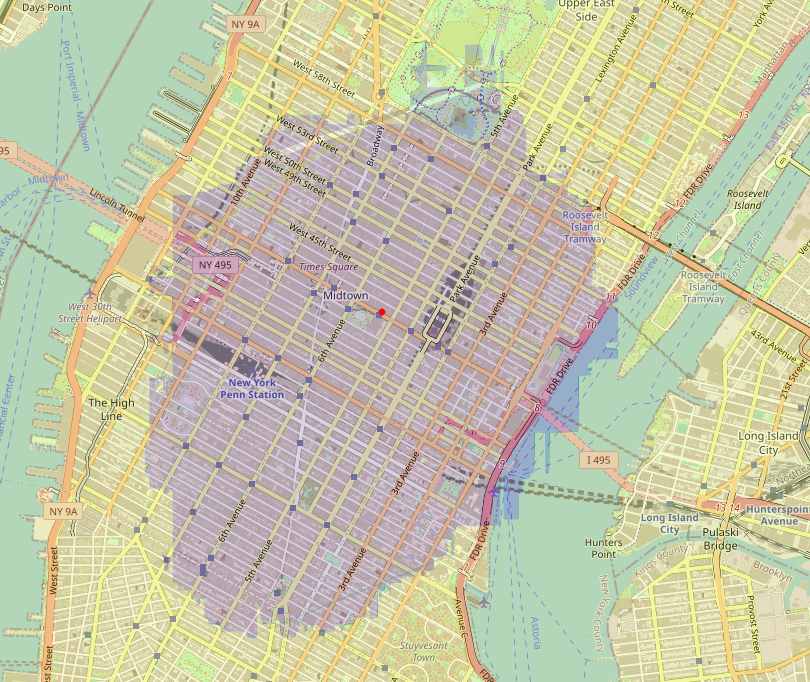
Here the blue region corresponds to where the model think we can reach driving in 5 minutes of driving, starting from the red point, an isochrone map. It’s significant that the model has learned such a realistic interpretation of the physical world - as travel time is mostly distance driven, it is intuitive that we’d see an area centered around the pickup point. Purely from the coordinate signal, the model has learned that this area is entirely homogenous, except near the border. This is quite remarkable, as generally for isochrone mapping you’d require a strong routing engine such as OSRM or Valhalla and an underlying road network graph.
We can sample arbitrary pickup points to make sure the good properties of the model are not caused simply from modelling the neighbourhood of the median well:
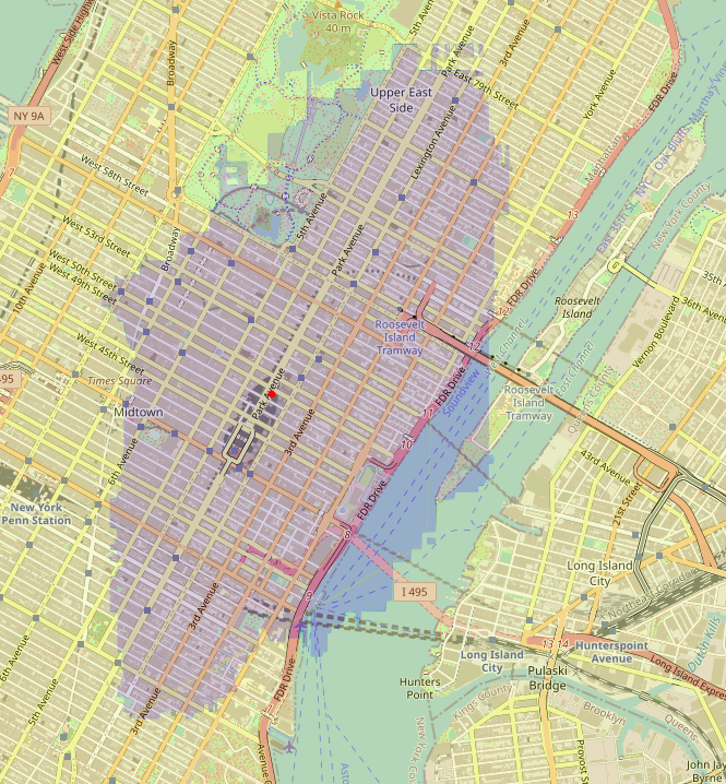
Here we see the model learning that driving towards Upper East Side on Park Avenue is faster than west-east, resulting in an oval-like isochrone.
And finally, we find a failure case:
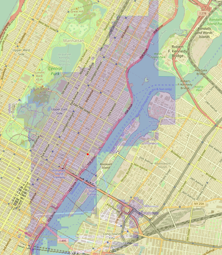 Here the model has correctly inferred that you can go over the bridge into Queens (and that area is blue), but we’d probably want it to understand that in this case the whole route to Queens should be blue. Most likely it’s caused by the fact that we don’t have a sufficient amount of trips with dropoff on the Queensboro bridge or near it :) We can also see that the horizontal-vertical split rule can look a bit clumsy.
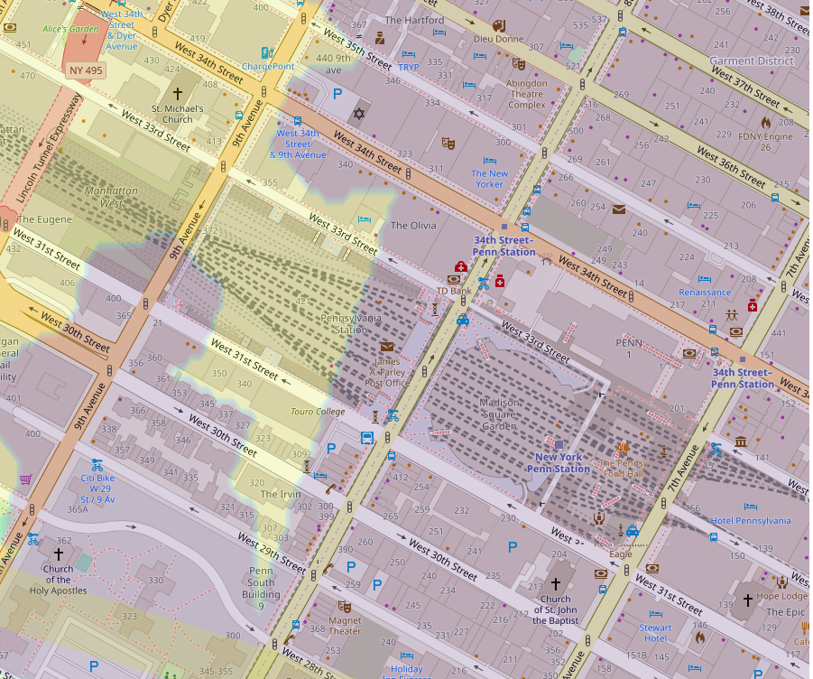
The corresponding decision boundary around the median pickup for embedded H3 model looks like this:
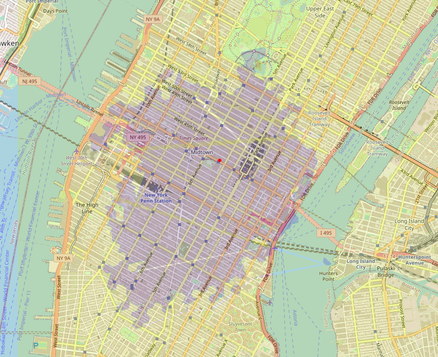
Indeed, the neural network model sees the map in hexagons, and we can recognize cell outlines straight away. Additionally, we see that the boundary looks less like a uniform blob we saw for the GBT, and capable of more complexity. This behaviour is intuitive, as GBT requires more splits to model exclusion (4 splits for square), while the H3 embedding based model can just turn any embedding’s key-value vector “on” to change the target prediction.
An interesting property of NYC the model seems to have learned - if I’m not overanalyzing this - is that getting to the area immediately behind (from the direction of the red point) Penn Station takes a longer time. As the busiest transportation facility in the Western Hemisphere, you’d certainly expect tough traffic there! With its horizontal/vertical splits and requiring multiple splits to model a neighbourhood, the GBT model has less incentive to capture this anomalous pocket and we see that on the GBT map there is no exception near Penn Station.
References
[1] TabNet: Attentive Interpretable Tabular Learning, Arik & Pfister, 2020
[2] On Embeddings for Numerical Features in Tabular Deep Learning, Gorishniy, Rubachev & Babenko, 2022
[3] How and why we built a custom gradient boosted-tree package, Lyft, 2021
[4] Gradient boosted decision tree neural network, Saberian, Delgado & Raimond, 2019
[5] Tabular Data: Deep Learning is Not All You Need, Shwartz-Ziv & Armon, 2021
[6] DeepETA, Uber, 2022