Quarterly planning is a noisy optimisation problem

Background

After working for 5 years on ML projects at Bolt, I was asked by my manager (only somewhat seriously) to give a farewell presentation on how to increase one’s impact as an individual contributor (IC) in a large product organisation. This got me thinking about how we measure, attribute and plan for impact in technology companies. One thing led to another and here we are, with Monte Carlo simulations for career impact. But there’s nothing like writing a simulator to prove fairly commonly known truths, right?

Senior IC (individual contributor) career path is still a relative novelty within the grand scheme of things. While the traditional approach to promotion pushes high performers into management path, where their individual impact becomes muddled and difficult to measure, ICs are evaluated on their raw contributions alone. Usually (at least in the ML field), this is measured in units of some business metric that their projects hopefully help to improve. Whether you like it or not, this sort of impact assessment is going on in the background each time promotions, salary reviews or re-organisations happen. So in order to maximise your overall impact in the organisation, it helps to understand how an organisation itself operates.

Problem setup

Most big technology companies operate on a quarterly planning cycle. Optimally solving this is equivalent to solving the knapsack problem - given a fixed resource count (usually denoted as human weeks), choose from a set of possible projects to maximise some business metric (usually revenue, GMV, profit etc).

A spreadsheet used for quarterly planning of a food delivery platform might look something like this:

Project	Description	Benefit	Cost	ROI (kEUR/w)
A	Fix payment button	500k EUR	2 human-weeks	250
B	Adopt new UI framework	275k EUR	5 human-weeks	55
C	Simplify restaurant on-boarding	630k EUR	6 human-weeks	105
D	New dispatching algorithm	2.5M EUR	13 human-weeks	192
…	…	…	…

With only one employee, we have 13 weeks available in a quarter. Given this constraint, it would be best to work only on project D, and nothing else.

We can extend this simple model by taking the engineer’s perspective into account. Instead of taking ranked roadmap items as a given (“just solving tickets”), it seems preferable to spend some effort to do research and re-assess the proposed items. That’s because the benefit and cost are not deterministic, they are only estimates for a random variable from some distribution.

Secondly, the benefits of a software project accrue into the future, rather than being a lump sum. Usually this scale with the business growth - we can think of project benefits relative to the overall revenue or profit. In an ideal world, cost is a one time thing - you build something and it just works - but realistically, there is some future maintenance cost of new features.

Finally, there’s a trade-off between implementation cost and future maintenance costs - we might decide to do things somewhat sloppily initially to ship faster. Then, in the future, we have the option to reduce the tech debt with further investment into the project.

Putting all of this together, the rational engineer would solve something like a dynamic stochastic knapsack problem with the additional choice variables for tech debt, research effort and refactoring. I’m not going to even bother with setting this up formally, let alone solving it, mostly because I doubt anyone in the real world does anything close to it. I’ve yet to see anyone take into account future maintenace costs of solutions in quarterly planning, not to mention how people dislike stochasticity. Instead, I simulate a few scenarios with baseline “sensible” strategies and see if they reveal anything about the trade-offs. What are these sensible strategies?

• not spending any effort on exploration vs spending some
• never taking on tech debt (purist) vs sometimes doing it (necessary evil)
• varying the overall level of recurrent maintenace cost (a proxy for engineering quality?)

Simulation

For the following, I wrote a simple simulator (code here) with the following conditions:

• Each quarter, there are $ N $ possible projects to work on, which have a random benefit (normal) and cost (log-normal). Log-normal distribution of costs is based on the interesting argument made by Erik Bern.
• The planner chooses the top K ones to work on that fit into the time budget, ranking them heuristically by initial benefit and cost ratio. These initial estimates are unbiased (more on this later).
• While projects keep accruing benefits every period, there is also some maintenance cost involved. However, this is not accounted for at project selection time.
• The maintenance cost is a function of initial project cost and how much tech debt was taken on implementation.
• Before choosing new projects, the planner can refactor existing projects to reduce their tech debt.
• Before choosing new projects, the planner can explore them in-depth, expanding time budget, but reducing the variation of benefit/cost estimates.
• Many arbitrary constants and heuristics - keep in mind this is just a thought exercise. 🙂

Let’s play around with the choice variables to see what would be a good strategy to approach this problem with.

Results

As a brief aside, note that there is a crucial difference in how we model the planner’s knowledge of the estimates of benefit and cost. Currently, we’re assuming that the planner has knowledge of the full distribution. To illustrate, consider having to choose the best 2 projects out of A, B and C with the following expected rewards (100K, 130K and 180K):

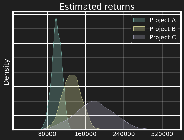
If we really know the full distribution (which here means the mean and variance), then it’s straightforward that we should pick B and C. However, this implies that the estimate in our planning spreadsheet is an unbiased estimate for the mean. For more complex distributions like the lognormal, we’d be assuming that our spreadsheet number corresponds to $ \mathbf{E}(x) = \exp \left( \mu + \frac{\sigma^2}{2} \right) $ with correct estimates for $\mu$ and $\sigma$! This seems highly suspect. It seems more likely that the number in our spreadsheet is only an imperfect estimate for $ \mathbf{E}(x) $. Perhaps we have worked on similar problems before, and can infer the mean based on historical data. In the absence of that, our estimate might be really noisy, though. We can model this extreme scenario by drawing the estimate as just one sample from the same distribution. This is the fundamental difference between known and unknown unknowns. If we know that a project will have a high variance of outcomes, we are still able to plan for it, taking the variance into account. If, however, both the mean and the variance we estimate are themselves noisy, then we run into the reversion to the mean problem. This is illustrated below, where for 100 time periods, we select top 5 projects from 20 randomly generated ones, and then compare the distribution of actual rewards to the estimated ones. Since we’re doing the selection on a random variable, likelihood of selecting an extreme value is increased. The variance of the estimates is significantly less due to the same reason.

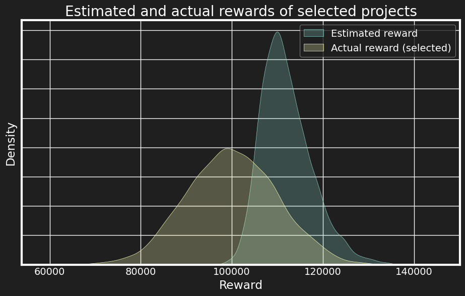
Real life is probably somewhere in-between of the known and unknown unknowns territory, so we should expect our spreadsheet ROI estimates to be overestimated, and our headcount budgets to often explode when dealing with uncertain projects. Note that this is not an artifact of the lognormal distribution, as here for rewards we used a normal one. The root cause of it is selection on a random variable.

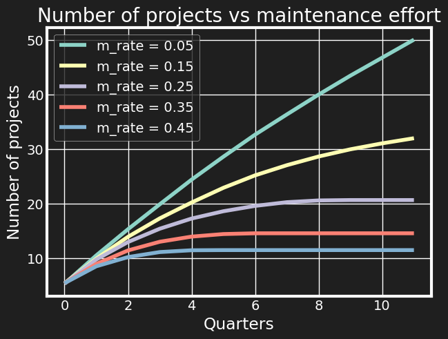
Coming back to the simulation model, the first thing that is fairly obvious is that if existing projects introduce maintenace costs, then the rate of shipping new things is going to slow down over time. So the main question becomes, how to keep up as high a pace as possible when juggling between new and old stuff. Here we compare the outcomes after 4 years for different rates of recurring cost, i.e. a fraction of initial development cost that needs to be spent each quarter just to keep something up and running.

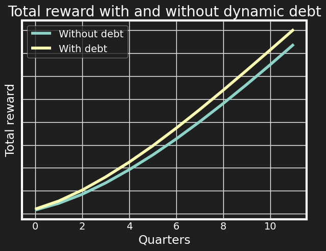
Similarly, we can plot the total reward for the cost rates.

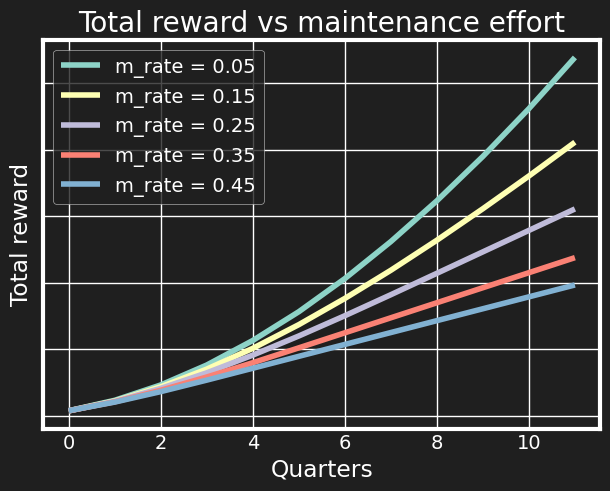
All the curves are exponentially growing - if you add more projects with a positive impact, you are adding on top of the impact of the projects you’re already maintaining. However, we see that the difference between outcomes is quite drastic. If we take the maintenance fraction to reflect the overall level of tech debt, then the first takeaway is that technical debt will need to be paid back, but it’s paid back from your own impact and career growth potential. Often I’ve seen tech debt arguments boil down to something like “will the system still scale in 5 years?” where the average engineer doesn’t care much about what happens after 5 years, but here we see it can start playing a role within the immediate tenure time as well.

Alternatively, we could view tech debt as a dynamic lever: there probably exists a successful strategy taking on tech debt when the (expected) value of current possible tasks is high and paying it off when the value is low. We could set some threshold on the average ROI expectation of this quarter’s projects and cut the corners if it’s high. Intuitively, in case of urgency (we are not likely to see as high expected rewards at other times), it makes sense to relax the quality standards somewhat, even if this locks in future productive resources into maintaining the horrible mess we’ve made. However, at times of low opportunity cost, we can spend time to fix it, to free up resources for future projects. While this provides another optimisation avenue, the winnings from this are generally much smaller than from being able to reduce your overall maintenance rate. This is because a) given enough projects, the budget is almost entirely exhausted by maintenance and tech debt adds to that cost by doing a noisy gamble on the reward, b) there is a very limited combination of parameters where taking on tech debt is more advantageous than not (because the full additional cost of tech debt is the increased maintenance cost and the eventual refactoring cost, unless we discount the future heavily (which we currently don’t do in the 12 quarter simulation)).

We’d have to make quite generous assumptions on how tech debt works to see a significant difference, for example with:

• Assuming x% of “cutting corners” reduces initial implementation cost by $x$%, and increases maintenance cost by only $\frac{x}{10}$%
• The refactoring/rewriting cost is just 30% of the initial implementation cost (unlikely!)

the results are not too different:

This could clearly look different with different parameters assumed, nonetheless, dynamic technical debt leveraging seems a second order effect compared to the overall maintenance rate one.

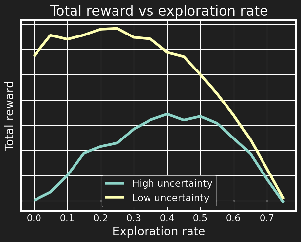
Finally, plotting the average outcomes over different values of exploration rate, the classic exploration-exploitation dilemma becomes visible: if we do too little exploration, then we become “ticket solvers” or just “building cool stuff”, while the opposite end of the spectrum is usually called “analysis paralysis”. There is a sweet spot which depends on the variance of the benefit/cost estimates and how much the exploration will reduce uncertainty. As expected, for a fixed level of rewards, higher uncertainty means higher required exploration rate, but also worse outcomes. I think the reason ML teams tend to spend more time on exploration is directly tied to the higher uncertainty of the nature of the projects. And clearly, you should only use ML when you expect high returns from a project.

What does this have to do with real life?

• Planning estimates are almost surely overly optimistic due to selection on noisy estimates. This is why hand wavy rules like “gut feeling estimates times 3” are often quite accurate, and provides another mechanism to explain budgeting failures, as this is not an artifact of the log-normal distribution only.
• Working on the right thing can often be more important than the work itself. The higher the uncertainty of a project (or alternatively, the more you can expect to reduce it), the more should be invested into this. This is why having dedicated data analysts for planning and impact estimation becomes important at scale.
• To increase your technical impact within an organisation, it’s important to not “get stuck” with poorly engineered legacy projects - 5% maintenance cost on average ships 80% more projects over 3 years than 15%. I’d wager that the number of successfully shipped projects might even be the best proxy for recognition, as people tend to be biased towards new and flashy projects.

Tangent on ML projects

While the above model is general enough to reflect any engineering projects, it’s worth pointing out that machine learning projects have some idiosyncracies:

• It’s possible that in your company there’s a separate team of data analysts for impact estimation (exploration), so it’s not the actual engineer doing impact estimations. However, it comes out of the company’s resource budget nonetheless. If we think of analysts as a leveraging factor on engineers, this resource might be better used elsewhere (opportunity costs). Quite often, especially in the ML/DS field, it is the engineers themselves who need to estimate the impact.
• Another way to write the estimate of monetary impact of a project is $dB = \frac{dB}{dA} \frac{dA}{dE} dE$ where dE denotes the effort spent, $\frac{dA}{dE}$ shows how much a model’s accuracy improves from the effort, and $\frac{dB}{dA}$ shows how much the business metric improves from the accuracy improvement. ML practicioners are in double trouble here: not only is it very hard to understand the effect on business metrics, often we don’t know how much a model can be improved until we actually try to do it.
• Probably the most useful uncertainty reduction tool I’ve encountered is building demos and sharing these with stakeholders ASAP. On the one hand, being able to ship something like this fast significantly reduces the effort estimate - especially given that ML tends to be viewed as “researchy” - while it also sets some lower bound on the rewards, at least the $\frac{dA}{dE}$ element.