Compressing images with neural networks

To see a World in a Grain of Sand
And a Heaven in a Wild Flower
Hold Infinity in the palm of your hand
And Eternity in an hour

William Blake

Introduction

Image and especially video compression is a problem of obvious real life significance, with video traffic taking up over 60% of all internet traffic. Increasingly better lossless and lossy codecs have been developed over the years to combat this problem. Relatively recently, a nascent research domain on using auto-encoder style neural networks for compression has emerged. This post goes through the evolution and highlights where the field might be heading.

JPEG

To understand neural compression, we first need to understand the ubiquitous JPEG standard which has been around since 1992. Lossless codecs exploit statistical redundancy in data: if you can predict the next byte conditional on the previous ones, then using the same statistical model in both encoder and decoder sides increases compression ratio by assigning smaller codes to more likely bytes. Lossy codecs go further by disregarding some “less important” data entirely.

There are many great tutorials on JPEG online, e.g. this, but the most important takeaway is that human eyes are much more receptive to low frequency changes such as edges than to high frequency changes such as elaborate textures. Artists exploit this by creating an “illusion of detail” instead of actually drawing every individual blade of grass.

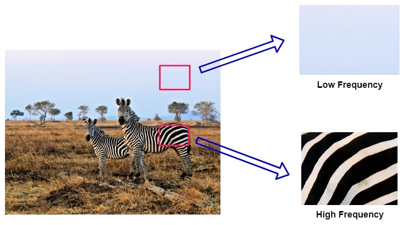Understanding frequency in images

JPEG exploits this by transforming the image data to the frequency domain using the discrete cosine transform, expressing each 8x8 pixel block of an image as a sum of cosine functions with different frequencies and amplitudes. Instead of $H \times W$ spatial pixels, we are left with $H \times W$ DCT coefficients, where each 8x8 block of coefficients corresponds to a block of the image.

Next, the 8x8 block of values is element-wise divided by an 8x8 quantisation table, and the results are rounded (this is what makes JPEG lossy). Intuitively, whenever you lower the quality setting when saving a JPEG file, this increases the values of the quantisation table, causing more zeros in the final representation of the image, making it easier to compress. It’s important to note that the values in the quantisation table are not uniform, nor random, they are carefully hand-picked to provide pleasing visual results. In fact, there is nothing special about these tables insofar as any software or user can change their values for desired effects.

The resulting quantised frequency values are the compressed representation of the image. In practice, this is further compressed with lossless encoding (all the rounded zeros are redundant), which we’ll skip this time. But what’s important to note is that DCT and quantisation are reversible operations, so we can do the inverse of them in the decoder stage, resulting in a lossy reconstruction of the original image.

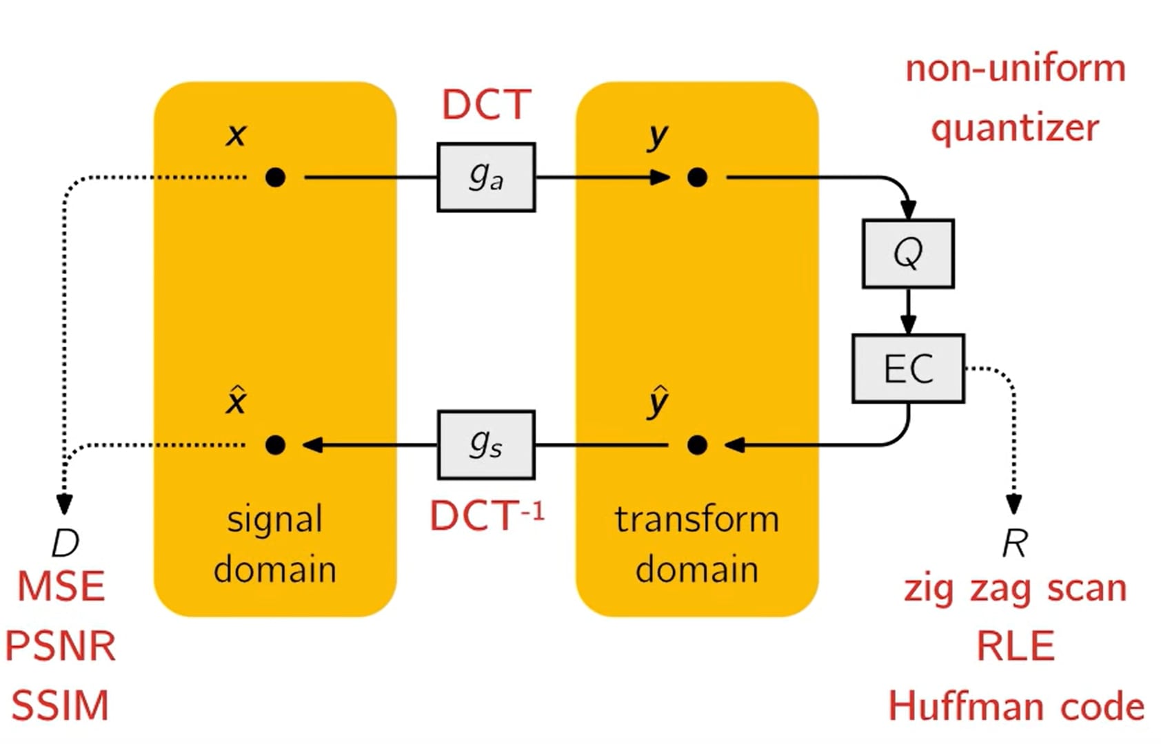High level diagram of JPEG internals

The above slide from Johannes Ballé’s 2018 talk summarises JPEG on a high level. It’s striking how closely this resembles a neural network diagram - we have a natural loss function and two (linear) transformations and their inverses. A natural question is whether such a system could be end-to-end trained by parametrising the transforms such as this:

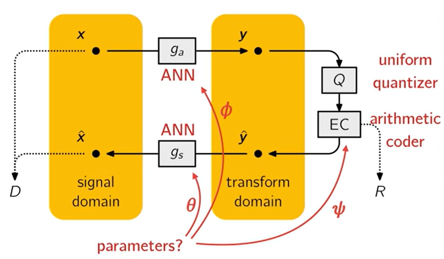High level diagram of learned image codec internals

Autoencoders galore

So why can’t we just train any autoencoder to minimise MSE and be done with? By projecting the image data to some low-dimensional bottleneck, we could use that directly as the encoded representation, right?

Bit embeddings

This is pretty much what the first iterations tried to do. For example, in [7] the authors moreover constrain the bottleneck to be a binary representation. This has the additional benefit that the vector can be directly serialised and bitrate can be estimated directly from the bottleneck size.

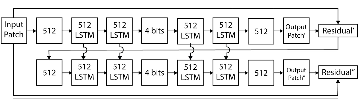Progressive bitwise encoding with LSTMs, [7]

Here, the autoencoder recursively generates a 4-bit (keep in mind the authors were compressing tiny 32x32 images!) representation of the image, with the residual of that reconstruction being fed into the next layer etc. By repeating this e.g. 16 times, we could generate a 64-bit vector to be transmitted to the receiver. This means the method is also one of the first to have adaptive rate control, which is a desireable property for a codec.

Unfortunately, it does not achieve the best compression ratios in practice. That’s because actual compression rates mostly depend on the Shannon entropy of the source file. Since this autoencoder has no incentive to reduce the entropy of the latent vector, we might not be compressing optimally in terms of the bitrate-distortion trade-off.

End-to-end training

A seminal breakthrough came in 2017 when [1] designed the first end-to-end trained model that directly optimises for the rate-distortion trade-off. Their key insights were the following:

• Using a loss of the form $L = R + \lambda D $, where R stands for bitrate and D for distortion (e.g. MSE), achieves an optimal trade-off between the two (for a given value of $\lambda$ moderating the weights).
• To estimate $ R $ by a neural network, we can use the fact that actual compression rates can be very close to actual entropy, so we only need to train a probabilistic model of our quantised latent variable $ \hat{y} = round(y) $ and the entropy of it gives the bitrate directly: $ L = -\mathbf{E}[\log_2 P_{\hat{y}}] + \lambda \mathbf{E}[D]$ where $P_{\hat{y}}$ is the probability distribution of $\hat{y}$. Note that both terms in the loss depend on the probability model, as $\hat{y}$ is also used for decoding the image.
• A specific type of lossless coding - adaptive arithmetic coding - is used to actually compress $ \hat{y} $ into a bitstream. Without going into too much detail, the key insight is that both the arithmetic encoder and decoder depend on the probability distribution of symbols (a symbol here is a possible value of $\hat{y}$).

This new model achieved better compression ratios than JPEG or even JPEG2000.

Hyperprior

Once the $ R + \lambda D $ loss became prevalent, it became clear that the best way improve compression rates is to improve the entropy (probability) estimation. Another way to look at this is through the arithmetic coder: imagine we were encoding English text. For the hackneyed example input “a quick brown fox jumps o”, if we use a static probability model, then the most likely next character is always space. However, if we had access to some GPT-style context-aware next character predictor, it could condition on the already available information and achieve far better compression ratios. Note that both the encoder and decoder would need to use the same model.

[2] does something similar. When the previous probability model was fixed (essentially reflecting the expected distribution of latents over all training set images), now we emit an additional quantised channel $\hat{z}$ that is also sent as bitstream. The receiving end then first decodes $ \hat{z} $, reconstructs the distributional parameters of $ y $ from it (in practice, each element $y_i$ is modelled as a Gaussian with), and then decodes $ \hat{y} $ conditional on these parameters, that means the probability model becomes image-specific.

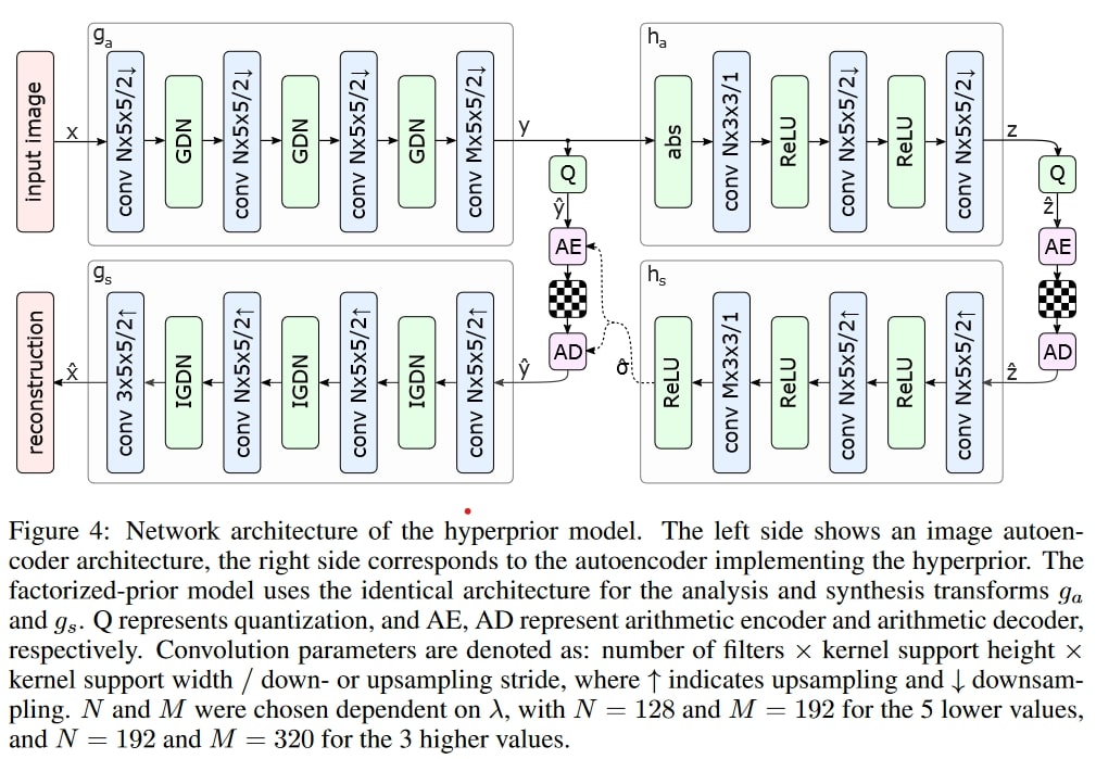Seminal hyperprior network, [2]. In the above, GDN is just some alternative non-linearity, ReLU could be used instead

I have played around a bit with the hyperprior model, using the popular CompressAI library - you can find a notebook here. Using a toy dataset of 100k 96x96 images (STL-10), I’m training a tiny toy model at different $ \lambda $ values and logging the average entropy and MSE loss for these. While this does is not yet enough to beat JPEG, it showcases how the rate-distortion training happens in practice.

Here are some fun images of a ram progressively improving during the training process:

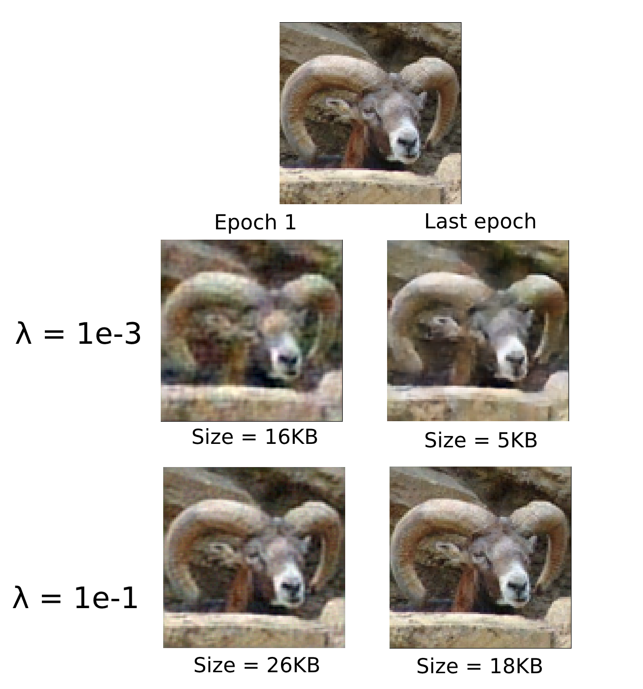Reconstructing a ram

As expected, a lower value of $ \lambda $ incentivises the model to focus on compression, while the higher one gives us a rather realistic reconstruction of the original image (top).

Autoregressive prior

The hyperprior showed that feeding additional information to the arithmetic coder’s probability model improves compression rates, namely sending image-specific $ \hat{z} $. But there is other information we are not using. For example, let’s say we are in the process of decoding $\hat{y}$ pixel-by-pixel. After the first half, it becomes clear that we have half of a dog. It is then very likely that the remaining half is the latter of the dog. We can update the probability model with this information - as long as both the encoder and decoder side do this kind of synchronised sequential processing, we can achieve a lower compression ratio.

This is pretty much the idea behind the autoregressive prior: instead of decoding all latents in one or two passes (like the hyperprior), we recursively predict the probability distribution of the next latent conditional on the previous ones. The arithmetic decoder can adapt in each iteration to optimally pack/unpack a single latent. In practice, instead of using all the previous latents, only a local neighbourhood (e.g. 5x5) of the pixel is used, which provides 12 pixels when serially processed:

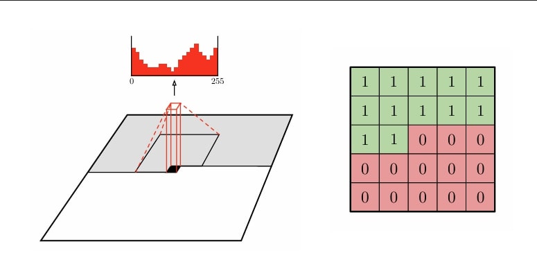Autoregressive image decoding [8]

This method added another step size improvement to learned image compression. Unfortunately, as you might be able to tell, iterating over the entire image pixel by pixel is really ineffective computationally. I recall seeing some papers where it was claimed that more than 95% of the decoding time was spent in the autoregressive model! This made the method mostly one of academic interest, used in competitions where only rate-distortion performance is measured, without computational constraints. Further work has tried to optimise this obvious bottleneck. For example, using something like the checkerboard context model can speed up decoding more than 40 times, without much of a drop in performance:

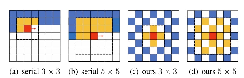Checkerboard context for arithmetic decoding [4]

Variable rate control

A glaring weakness of models trained for the $ R + \lambda D $ loss is that we need to train a separate model for each point of the rate-distortion curve. That would mean that if you are streaming video, the service would need to have N different models in storage ready to store, depending on your (dynamic) bandwidth - which is absurd. Traditional codecs can adapt rate on the fly, like the quality setting in JPEG.

Luckily, there’s a nifty little trick to support variable rate within one model. It’s fairly obvious that to support this, we should use variable values of $ \lambda $ during training, but these should be coupled with some input feature that tells the model which rate-distortion regime we are in. In [3], this is done quite elegantly by introducing a “gain” unit and its inverse. This is a learnable embedding-like vector that multiplies the encoded latent $y$ before it goes into quantisation - decoding performs the opposite.

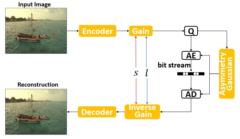Learned variable rate control [3]

If we recall JPEG, this is very similar to using different quantisation tables for different desired quality values, except it has the added benefit that the gain and inverse gain coefficients are trained end to end. During training, we can discretise the range of $\lambda$ and gain vectors, say to 100 values. Each sample gets assigned a uniformly random index in 100, and uses the corresponding gain vectors and $\lambda$ coefficient. In inference, we can then vary which of the 100 gain vectors we wish to use, and due to the way they have been trained, we effictively have a 1-100 quality index like JPEG!

Perceptual losses

In image reconstruction, pixel-wise MSE is usually used as the first simple loss function. However, this causes unwanted artifacts at low bitrates: let’s say you have a perfect reconstruction of the image but it’s shifted 5 pixels to the right. MSE would incentivise the model to prefer a blended nothingness over such slightly misaligned reconstructions. This would cause the model to blend out fine textures at low bitrates. Due to this and other issues, the MSE-based PSNR loss metric does not achieve high correlation to actual golden truth subjective test scores, unlike other more advanced metrics such as VMAF. A fun fact is that VMAF has won an Emmy award for technology and engineering :)

What are some of the more perceptual loss functions that have been used? One fairly simple improvement is weighting MSE by a saliency map of the input: it’s reasonable to assume that viewers care more about the reconstruction quality of human faces compared to minute background details. Moreover, the pixel-wise L1 loss and Charbonnier loss have been tried to reduce blurring artifacts caused by MSE.

Since deep neural networks extract semantic information from images during their training process, it’s possible to pass through images through a pretrained network, extract deep feature activations and compare their distances to get a semantic similarity measure. This is what the PIPS loss does, originally using the VGG network for extracting deep features.

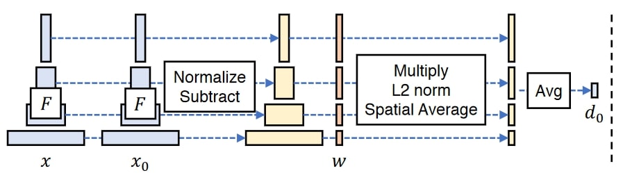PIPS feature similarity [9]

A similar alternative to PIPS loss is the style loss borrowed from the style transfer literature. It similarly extracts intermediate layer activations from a pretrained network such as VGG, but the metric is calculated in a somewhat different way, focusing on global statistics of the feature maps, meant to measure differences in style.

In [2], the authors show that image compression methods can be thought of as generative variational autoencoders as $ \lambda \to \infty$. It is therefore not surprising that many methods that have been useful in that field, have also been adopted in image compression. Another NeurIPS paper [5] showed that using a classic image generation method, a GAN discriminator, is useful for training the image compression model. In fact, based on human evaluations, a model trained for joint MSE, LPIPS and GAN loss was deemed better than BPG (a then state of the art image compressor based on the HEVC video codec) at half the bitrate.

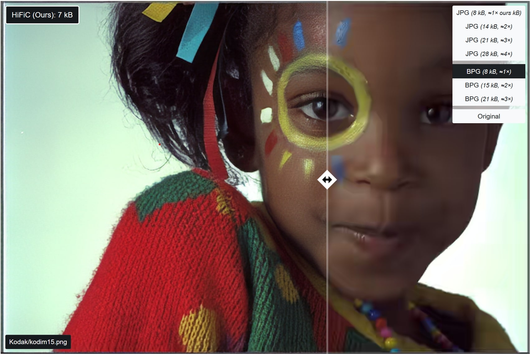HiFiC [5] vs BPG at similar file size

Challenges

Comparison of image codecs, CompressAI

The above image from CompressAI shows the progress of various learned image codecs against their traditional benchmarks, such as VTM, AV1, BPG. While these codecs are already somewhat outdated, it’s visible that generally the best learned and traditional codecs are neck and neck.

This is confirmed by the CLIC compression challenge where especially in the video track, winning submissions are often hybrid approaches where a traditional codec is combined with a neural post-processing layer (in-loop filter). The efficacy of such ensemble methods shows that neural methods do not dominate sufficiently to make traditional codecs obsolote. In fact, it seems that in the recent CLIC2024 competition, both the image and video track winners used the state of the art ECM codec.

But more than accuracy, the main concern of ML codecs is their computational cost, highlighted best by this concluding slide of the CLIC2022 challenge:

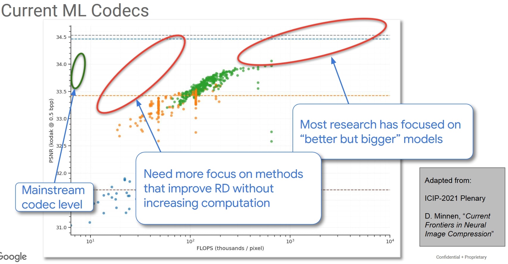Challenges in incorporating ML in a mainstream nextgen video codec

We see the difference between mainstream codecs and learned ones can be up to two orders of magnitude in the number of calculations. In the CLIC challenge, it’s common to see neural codecs have 10x longer decoding times, even if their inference can be run on a GPU.

Due to this, it might mean that at least for the time being, more lightweight hybrid neural approaches are the best way to enhance image and video compression. Although, it also seems likely that in the long run due to the bitter lesson effects, neural codecs which are significantly simpler conceptually (JVET codec documentation can easily span hunderds of pages :)) and meant to run on generic neural hardware (which is becoming more common) will prevail. At least it seems safe to predict that a good compression system will have at least some learned components in the future.

References

[1] Ballé, Johannes, et al. “Variational image compression with a scale hyperprior.” arXiv preprint arXiv:1802.01436 (2018).

[2] Ballé, Johannes, Valero Laparra, and Eero P. Simoncelli. “End-to-end optimized image compression.” arXiv preprint arXiv:1611.01704 (2016).

[3] Cui, Ze, et al. “Asymmetric gained deep image compression with continuous rate adaptation.” Proceedings of the IEEE/CVF Conference on Computer Vision and Pattern Recognition. 2021.

[4] He, Dailan, et al. “Checkerboard context model for efficient learned image compression.” Proceedings of the IEEE/CVF Conference on Computer Vision and Pattern Recognition. 2021.

[5] Mentzer, Fabian, et al. “High-fidelity generative image compression.” Advances in Neural Information Processing Systems 33 (2020): 11913-11924.

[6] Minnen, David, Johannes Ballé, and George D. Toderici. “Joint autoregressive and hierarchical priors for learned image compression.” Advances in neural information processing systems 31 (2018).

[7] Toderici, George, et al. “Variable rate image compression with recurrent neural networks.” arXiv preprint arXiv:1511.06085 (2015).

[8] Van den Oord, Aaron, et al. “Conditional image generation with pixelcnn decoders.” Advances in neural information processing systems 29 (2016).

[9] Zhang, Richard, et al. “The unreasonable effectiveness of deep features as a perceptual metric.” Proceedings of the IEEE conference on computer vision and pattern recognition. 2018.